Conditional Formatting In Pivot Table

In order to insert a pivot table we follow these steps. This displays the PivotTable Tools tab on the ribbon.

Abc Analysis Using Conditional Formatting In Excel Pakaccountants Com Excel Tutorials Excel Analysis

Conditional Formatting is commonly used to highlight data fields to easily identify outliers or narrow down the results.

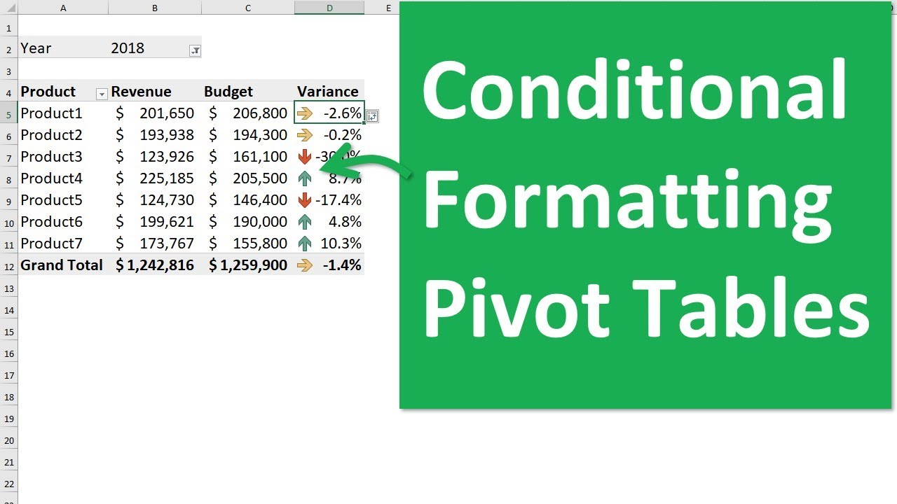
Conditional formatting in pivot table. In the example shown there are two rules applied. It can also add icons and data bars to the cells. The green shows the.

Working with pivot table that has conditional formatting. Format Cells dialog box will open. Conditional Formatting can change the font fill and border colors of cells.

This is great for interactive pivot tables where the values might change based on a filter or slicer. Name column B Month column C Orders column D and Sales column E. Then select Format only cells that contain.

When you use conditional formatting in your pivot it works as dynamic formatting. For more information see Apply conditional formatting. Select the cells.

For example say the conditional formatting needed to be a heat map or reach row label. If X criteria are true then Y formatting will be applied. There are three methods for scoping the conditional format of fields in the Values area.

Pivot table conditional formatting To apply conditional formatting to a pivot table create a new conditional formatting rule and pay particular attention to the apply rule to settings as described below. In addition to selecting the Preserve cell formatting on update option there are some choices you can make while setting up conditional formatting rules for a PivotTable that will affect the way the formatting is handled when the Pivot layout is changed expandedcollapsedfiltered. Httpscuttlyup4excel1927MFD Dont add conditional formatting to your pivot table before you see this.

In the Home Tab in the Styles Section click on Conditional Formatting and a dialog box pops up. I think the simplest solution is a very simple macro assuming you are ok with re-entering the rules for your conditional formatting. Unfortunately pivot tables have their own formatting which will overwrite your formatting until you specifically tell it otherwise.

Pivot Table Conditional Formatting In Excel you can use conditional formatting to highlight cells based on a set of rules. This excel feature also works on the Pivot Table in a similar way. Select containing and then enter blank.

It can apply multiple conditions to a single cell or an entire array. Our table consists of four columns. In above pivot table you have applied conditional formatting to highlight the cell with the highest value.

However you need to set the correct option from the pivot tables formatting options. Whenever you filter values or change data it will automatically get updated with that change. First let us insert a pivot table using our data.

Keep your conditional fo. There are a variety of rules to be applied in the pivot table. We are not going to program a macro in VBA just use the macro recorder.

Using this feature you can specify some condition and excel would format the cell only if the condition gets fulfills. Go to Conditional formatting tab. Conditional Formatting in the Pivot Table To apply Conditional Formatting in any pivot table first select the pivot and then from the Home menu tab select any of the conditional formatting options.

Pivot Tables are also dynamic elements and conditional formatting rules. So under Browning there is Farm and Surgery. Select specific text from the dropdown list of format only cells with.

In the PivotTable select the field of interest. Insert a pivot table. Select the New rule option.

By selection by corresponding field and by value field. All the conditional formatting is based on IF -then logic. Now to apply conditional formatting in the pivot table.

However this feature works a bit differently when dealing with a Pivot Table. If the Conditional Formatting was a color scale and it was only applied to each row label. First select the column to format in this example select Grand Total Column.

How can you apply the conditional formatting to the pivot table in order to automatically apply it to new rows. Then click on Numbers Custom. And then click OK to close this dialog and now when you format your pivot table and refresh it.

In the PivotTable Options dialog box click Layout Format tab and then check Preserve cell formatting on update item under the Format section see screenshot. Click on New Rule and another dialog box pops up. Conditional Formatting in Pivot Table Based on Built-in Presets To apply conditional formatting in a pivot table you need to select a group of cells and apply a conditional formatting rule.

Select the Pivot table area. For example highlight the cells that are above average or lower than a specific amount. If you want to format the data with Above Average values under TopBottom Rules choose the option.

Change the number format for a field. The formatting will also be applied when the values of cells change. Here a few essential points that everyone should know while using Conditional Formatting in the Pivot Table.

Conditional Formatting is a very common excel feature that is used to format the cell or cell values based on user-defined conditions.

Pin On Teaching

Use This Complete Guide To Learn How To Use Conditional Formatting In Pivot Pivot Table How To Apply Learning

How To Use Conditional Formatting In Google Sheets Google Sheets Google Tricks Remote Teaching

Pin On Excel

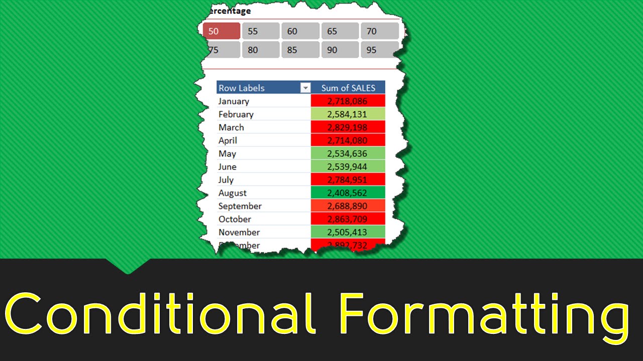
Creating Heat Maps From Excel Pivot Tables With Conditional Formatting Pivot Table Excel Pivot Table Heat Map

Basic Conditional Formatting In Excel Access Using A Sales Example Exceldemy Excel Microsoft Excel Data Bar

5 Pivot Tables You Probably Haven T Seen Before Exceljet Pivot Table Report Templates Excel

Intro To Pivot Tables And Dashboards Video Series 3 Of 3 Pivot Table Excel How To Apply

Search Highlight Data Using Conditional Formatting In Excel Excel Tutorials Excel Excel Spreadsheets

Applying Conditional Formatting To A Pivot Table In Excel Pivot Table How To Apply Pivot Table Excel

Pin On Excel Shortcuts

How To Apply Conditional Formatting To An Excel Pivot Table Youtube Pivot Table How To Apply Excel Spreadsheets

Pin On Tech

Pin On Excel Pivot Tables And Slicers

Excel Certified Data Validation Chain Management Pivot Table

Applying Conditional Formatting To A Pivot Table In Excel Pivot Table Pivot Table Excel Excel

Make Pertinent Data In Your Pivot Tables Stand Out With Specialized Formatting That Is Autmatically Applied When You Set How To Apply Online Student Job Seeker

10 13 Control Conditional Formatting With Excel Pivot Table Slicers Excel Tutorials Pivot Table Pivot Table Excel

Create Count Of Colour Cells In Conditionally Formatted Sheet Cell Excel Projects To Try